Today, Motorola is one of the most respected communications brands in the world, but in 1986, the company faced some serious challenges. It was struggling to compete with foreign manufacturers, and its own vice president of sales admitted that the quality of its products was pretty poor. So, then-CEO Bob Galvin set an ambitious goal: Achieve tenfold improvement in product quality and customer satisfaction in five years. But how? The plan focused on global competitiveness, participative management and, most importantly, stringent quality improvement.
Advertisement
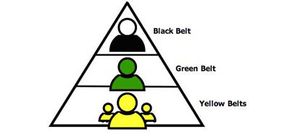
Motorola quality engineer Bill Smith dubbed the quality improvement process Six Sigma. It was a catchy name, and the results were even more striking. In 1988, Motorola won the Malcolm Baldridge National Quality Award based on the results it had obtained in just two years. Now, more than two decades later, thousands of companies use Six Sigma to optimize business processes and increase profitability. In fact, an entire industry has grown up around Six Sigma: Motorola offers extensive training through Motorola University, an army of experts called Black Belts travels the globe helping organizations set up and run Six Sigma projects, and hundreds of books about Six Sigma have been published.
One might think that, given the time and resources dedicated to it, Six Sigma would be too complicated for the layperson to understand. Not true. At its core, Six Sigma is a relatively simple concept to grasp -- which we'll demonstrate in this article by answering the following basic questions:
- What is Six Sigma?
- When was it developed?
- How is it implemented?
- Where is it used?
Advertisement